Celestial Mechanics - How Gauss Solved It

What information did Gauss have to begin?

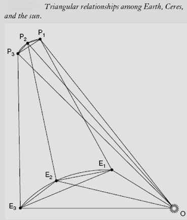
The Earth’s orbit was well known by the time of Gauss. So at the particular times of Piazzi’s observations, the observer’s position was known.

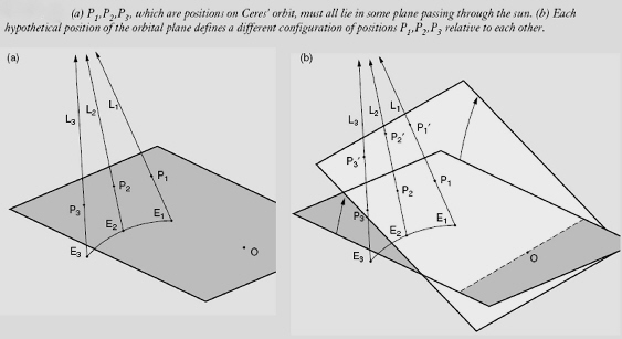
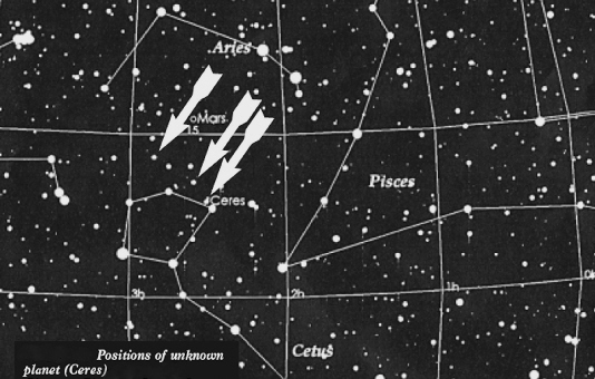
Gauss realized that these observations represented lines of sight for particular times. Therefore, Ceres must have lay somewhere along each sight line at the time of each observation. What was missing was to know how far away Ceres was.

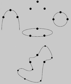
The problem at first appears very difficult because an infinite number of curves may pass through 3 points.

Other astronomers considered the problem intractable because of the small number of observations made, and the small area of sky (<9 degrees) traced by all the observations. But for Gauss’ method, he needed only three observations, and the small span of the observations did not impede his approach.

If you would like to know about the times of his three chosen observations, look here.

Gauss made the assumption that Ceres followed a Keplerian orbit. Therefore, the sun was at one foci, and the plane of Ceres’ orbit would intersect with the plane of the Earth’s orbit along a line passing through the sun.

In the drawing, the sun is at point O. The observations on Earth are from points E1, E2, and E3. The Lines of sight to the 3 observed positions of Ceres are L1, L2, and L3. At the times of the observations, Ceres is at points P1, P2, and P3, but the distances from E1, E2, and E3 are unknown.

 At this point, Gauss brought Kepler’s Second Law into play. Ceres must follow an ellipse in a plane with the sun at one foci, for which the arc of Ceres sweeps out equal areas in equal times.

One key point is that Gauss realized that the ellipse imposed an order on the entire arc of Ceres’ orbit. Moreover, no two arcs sweeping out identical area are exactly super-imposable in any of their parts. Each arc is uniquely characteristic of the ellipse of which it is a part.

 
An analogy can be made to the catenary. A catenary is defined by the two endpoints. Once those are defined, every part of the arc between (up to the suspension points) is implicitly given. Or alternatively, the entire form of the catenary is implicitly determined by any of its arcs, however small.

Try to experiment with this idea on a catenary. You can use a hanging chain to play with this concept. The tension on the hanging chain also is uniquely determined by each point on the catenary.

 Back to our geometric drawing. We may draw the arcs swept out by Ceres’ motion between points P1 and P2, and P2 and P3, on our (still hypothetical) ellipse. Remember, Gauss did not yet know where the points P1, P2, and P3 lay along the lines of sight. That is, for example, he did not know the distance E2P2 (that defines the distance of Ceres from the Earth at the second observation). Therefore the angles of orientation of the plane of Cere’s orbit (i, theta, and phi) were still unknown. But he did know that the sectors swept out (here, S12 and S23) must sweep out equal areas. (Of course, the time of the given observations were not exactly spaced so that t12≠t23; Gauss used ratios to adjust these values for comparability.)

Gauss’ key idea was that the conditions imposed by Kepler’s Second Law (Ceres’ orbit was an ellipse with the sun at one foci, and equal areas are swept out in equal times), together with the lines of sight, resulted in a very limited set of values for the five orbital parameters. The five orbital parameters, recall, uniquely define the 3 dimensions of the angle of the plane of Ceres’ orbit (compared to the plane of Earth’s orbit), and the shape of the ellipse itself.

One critical requirement in Gauss’ method is that the areas swept out (S12 and S23) must be estimated very accurately. Because the angle between the planes of Earth’s orbit and of Ceres’ orbit is shallow (as is typical in practice for most celestial objects), small errors in the area of the sectors result in large errors in estimating the position of Ceres. Gauss estimated the area of the sectors not only with simple triangles, but he then further refined this estimate.

Gauss computed a correction factor (still in use today) to adjust from the areas of the triangles T12, T23, T13, to the approximate sector areas S12, S23, S13. One form of the correction factor is:

 The rest, as they say, is history. Gauss became famous when Ceres was found very close to his predicted coordinates (which were distant from the predictions of other astronomers). Gauss’ method is still used today.

 Okay, now you really deserve to play with the model again!

Much thanks in particular goes to Bruce Director and Jonathan Tennenbaum , How Gauss Determined the Orbit of Ceres (Printed in The American Almanac, December 15 and 22, 1997), found at  http://american_almanac.tripod.com/ceres.htm